“This is cool, really cool, but I feel like maybe you need an intervention” – Friend’s reaction when I showed them this.
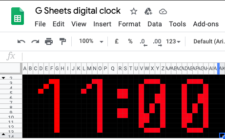
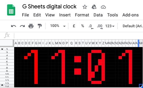
What have I done?
Using only Google Sheets formulas I’ve made a digital clock. It updates every minute, it’s a clock, that’s pretty much it.
Why have I done it?
I’m a very strong believer in getting the most out of the tools available to us and this kind of rubbish is a great way to learn things which are way more useful elsewhere!
Without doing anything like custom functions in JavaScript – Google Sheets is amazingly flexible. I’ve used it to automate things like project management tasks and even website change detection using Screaming Frog.
Google Sheets is also really accessible – if you make something in Google Sheets you can share it with colleagues and clients without them needing to install anything, without them needing an account, and without them being made nervous by any mention of code.
Languages like Python and JavaScript are great ways to get things done but it is fun to see what we can achieve with little ole Sheets.
The sheet
Access the Google Sheets digital clock here if you want to have a play with it. I’ve set the link to automatically copy so you have your own version where you can see the formulas at work.
How have I done it? (The important bit!)
As I say – the value of these things is what we are able to learn. So let’s see what we’ve learned.
1. Getting the current time – now()
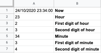
=now() returns current date and time in this format: 24/10/2020 23:24:00

We’ll put that in cell A1.
2. Getting minutes and hours – hour() and minute()
=hour(A1) will give us the hour contained in a specific time. If we used hour() on the timestamp above we would get 23
=minute(A1) gives us the minute. If we used minute() on the timestamp above we’d get 24

3. Splitting minutes and hours into individual digits – regexextract()
=regexextract() lets us get part of the value out of a cell, but only as long as it’s used on text (digits can be interpreted as either numbers or text in Sheets). So first we use =text(hour(A1),”##”) – that takes the hour from the timestamp and turn it into text.
You may notice below that the hour and minute values are left-aligned rather than right-aligned. That’s one way to spot whether Sheets might be treating digits as a number or as text.

Then we use =regexextract() to get the first number of the hour like so =regexextract(text(HOUR(A1),”##”),”^\d”). Don’t worry too much about that RegEx, all it means is “the first digit”. If you want to learn more about RegEx – check out my RegEx learning game – Slash Escape.
We’ll extract the last number of the hour like this; =regexextract(text(HOUR(A1),”##”),”\d$”)
Then we do the same for both of the minute digits.
3. Changing colours – Sheets conditional formatting
To create our digital clock, we need to tell sheets which cells to highlight at which time. To do that we’ll use Sheets’ amazingly flexible conditional formatting.
We’ll apply a different conditional format to each space in our clock. To make it clearer – here’s each of them highlighted in a different colour.
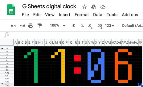
We have four rules, one for each digit in our clock. Each splits out a portion of the time for our display. Our broad process is;
- The rule defining the green number above
- When the first digit of the hour is 1 – highlight all the cells in the first block which we’ve marked as “1 cells”
- When the first digit of the hour is 8 – highlight all the cells in the first block which we’ve marked as “8 cells”
- The rule defining the blue number above
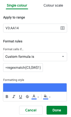
- When the first digit of the minute is 6 – highlight all the cells in the last block which we’ve marked as “6 cells”
etc. etc. etc.
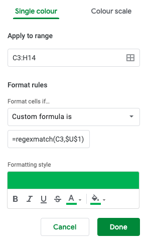

Our first, green digit, at maximum will occupy any of the cells between C3 and H14.
In each of the cells in that range, we’ve written out a RegEx which tells us if a digit will use that cell.
For example, cell C3 will be highlighted if we are creating the digits 4, 5 or 7. It won’t be highlighted if we’re creating the digits 0, 1, 2, 3, 6, 8, or 9. So in C3 we have written ^(4|5|7)$ which means “match 4, 5, or 7, exactly – nothing else.
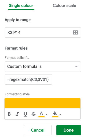
In this case – U1 is where we’ve put our first extracted digit of the hour. So the custom formula written there means “when the first digit of the hour matches 4, 5, or 7, highlight C3”.
One smart thing about custom formulas in Google Sheets is, if you apply it to a range of cells (like C3:H14) it will take relative and absolute cell references into account. In our formula we’ve used $U$1 – that’s an absolute cell reference – no matter where we are applying this custom formula – that part will always refer to U1. However – we haven’t written $C$3 – we’ve just written C3. So, in the first cell of our range, we’ll refer to C3 but if we apply this formula to a cell one row down it’ll refer to C4, if we then move one column across it’ll refer to D4.
This is how we create our clock without having to write out a different conditional formula for each one. When the conditional formatting is applied to C4, it’ll check whether the regex in C4 matches the first digit of the hour. The regex in C4 is ^(2|3|4|5|6|8|9|0)$ so if the first digit of the hour is 2 – C4 will be highlighted and C3 won’t be.
4. Drawing all the numbers – join()
It would be a massive pain to just try to write out all of these regex formulas one-by-one. Instead we’ll write out each of the possible digits we want to represent and then combine them into our regex.
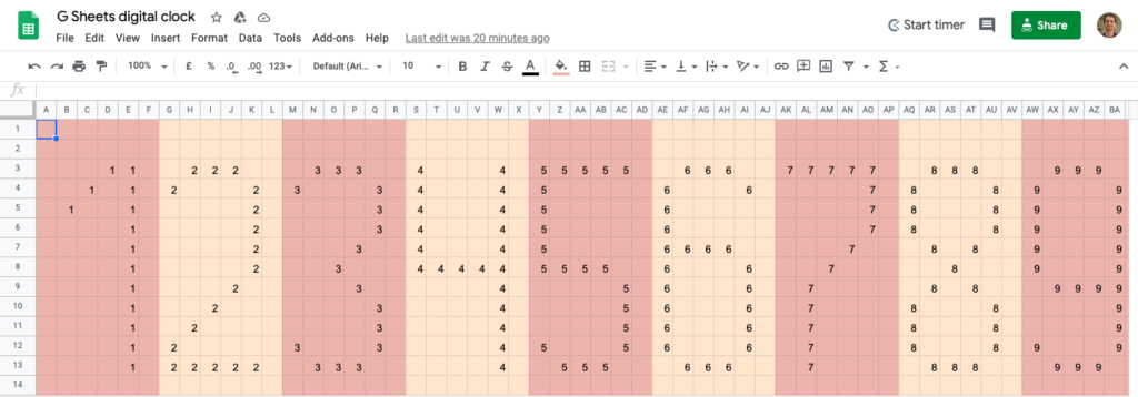

Our Clock C3 cell in our is a combination of the numbers in our digits sheet A3, G3, M3, S3, Y3, AE3, AK3, AQ3, AW3, BC3. Clock C4 is A4, G4, M4 etc. etc. etc.
The formula we use to do that is; JOIN(“|”,Digits!A3,Digits!G3,Digits!M3,Digits!S3,Digits!Y3,Digits!AE3,Digits!AK3,Digits!AQ3,Digits!AW3,Digits!BC3)
Basically – take the value from each of these cells and join them together with a pipe | in between them (because pipe in regex means or).
5. Removing errant pipes – regexreplace()
The problem with this is we have some empty cells so we can end up with a regex that reads |||4|5||7||| – having those empty spaces means we won’t just match numbers – we’ll match a lack of number too, which could screw up our clock. To get rid of those problematic extra bits we’ll use regex on our regex.


=regexreplace(JOIN(…),”\|{2,}”,”|”)
This formula will take the result of our join, identify anything that matches \|{2,} (basically two or more pipes in the row) and replaces them with | – one pipe.
We also don’t want to end up with pipes at the start or end like this; |4|5| so we’ll regexreplace on our regexreplace


=regexreplace(regexreplace(…),”(^\||\|$)”,””))
This formula will look at the result of our last regexreplace(), find anything that matches ^\| (a pipe at the start of the text) or \|$ (a pipe at the end of the text) and replace either with “” (nothing).
So now we have a regex like this; 4|5
5. Complete our regex – & concatenation
To make sure we have a nice, specific, regex to match on we can add some text to the start and end. Google Sheets has a concatenate function but I find using & easier to read
=”^(“®exreplace(…)&”)$”
That formula will take our cleaned up regex, add brakcets and a “start’ and “end” symbol so we have something like this; ^(4|5)$
We know that regex will only match either the digit 4 or the digit 5 and nothing else. Nice and specific.
6. Create all the rest of our digits – arrayformula()
At this point we’ve created the template for our first hour digit. We don’t want to go through all of that for each of the other templates and they can all be identical. So we use arrayformula to copy one block of cells to another place.
=arrayformula($C$3:$H$14) duplicates our template, we can do that for each of our other digits.
7. Highlighting the rest of our digits – Sheets conditional formatting


Our first conditional formatting formula checked each cell in the green block against the first digit of the current hour. Our second formula checks the cells in the yellow block against the second digit of the hour, our third block checks the cells in the blue block against the first digit of the minute etc. etc.
Any ideas?
As above – feel free to play around with the Google Sheet and see how it works.
This is a bit of fun which hopefully helps you learn some Sheets tricks that’ll be valuable elsewhere. One thing I love about open platforms like sheets is there are loads of people creating this kind of thing. When I started to share this, a colleague pointed out that Ben Collins actually created a working analogue clock using Sheets sparkline formulas, which is very impressive.
Have you seen any cool sheets projects recently? Anything you think I could have done better here? Tweet me @robinlord8
